We have been speaking so far of how to think systemically and/or how to explore the connection between behavior and structure in complex systems. We have also hinted to the fact that we live our lives while continuously immersed in or dealing with a multiplicity of systems and very often interact with systems that display circular causal relationships (feedback loops).
As already explained, feedback occurs when a consequence of an action comes to (retroactively) influence the action itself (the cause). Such circularity is at the root of the non-linearity and complexity of systems’ behavior; hence, it constitutes the greatest difficulty when trying to fully understand how a system works. Our mind has been prepared (through years of such an approach from the early school years) to seek and understand causal relationships only through linear sequences of cause and effect; thus, circularity makes us lose our bearings: comes the chicken or the egg first?
By now we know that the behavior of a system is determined by the systems’ structure, so studying such a structure and identifying the existing feedbacks and distinguishing the types of feedback in a system constitutes a first step in understanding a system’s behavior.
To do this, there is a graphic convention and a "visual language" that facilitates understanding and communicating how the system works: causal loop diagram (Cavana & Mares, 2004).
Here are some examples related to systems that we encounter in our everyday life and that explain how to see such systems (or situations) under a systemic perspective.
Positive Feedback Loop: couple crisis escalation
An interesting example that explains certain escalation dynamics in the tense relationship of a couple, is also useful to explain the so-called endogenous perspective introduced by Systems Thinking, as opposed to the “exogenous” perspective, for which a problem is always seen as motivated and due to causes that are external to the system (or our context of relevance – i.e.: our company is not working due to market problems).
Let’s then consider the story of Sam & Pam, husband and wife, living together for many years now.
From Pam’s recounting of their relationship, Sam is recently always mean to hear, without reason… it’s all his fault… If he was nicer to her, Pam’s life would be better.
In causal terms, this statement could be resumed by the following causal relationship:
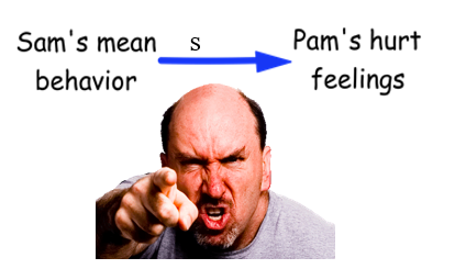
Figure 1: Exogenous perspective (“s” = same direction, in blue also for coloring purposes)
This graphical representation, as known, puts into direct causal relation (the small “s” stands for “same” direction of causality) the two statements (or “variables”) “Sam’s mean behavior” and “Pam’s hurt feelings”. This is also read as follows: the more Sam is mean to Pam, the more Pam’s feelings are hurt (so a growth in Sam’s mean behavior implies/causes a growth in the way Pam is hurt in her feelings).
However, if we put ourselves into an endogenous view and try to analyze the way this relationship works with a wider perspective, we might find that maybe there is also something that Pam is doing…
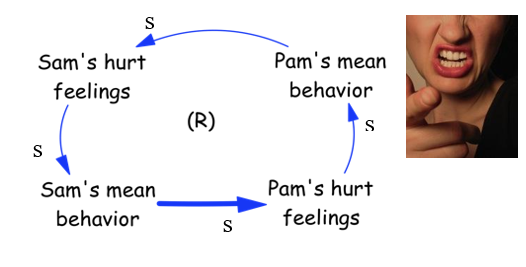
Figure 2: Endogenous perspective and reinforcing (R) feedback loop
We see in fact that as Pam gets hurt in her feelings, she also starts to be mean to Sam, which in turn causes Sam’s feelings to be hurt… And as soon as Sam’s feelings are hurt, he starts to be meaner to Pam…
The direct relationship between mean behavior and hurt feeling is the same, but we also have introduced another direct relationship (always in blue) between hurt feelings and the insurgence of a mean behavior. So the more feelings are hurt, the more the hurt person starts to be mean towards the other. The endogenous perspective lets us realize (in this specific case) that there is a circular relationship in action, which in the specific case is called as “reinforcing”, since the closed loop is composed by a chain of relationship acting all in the same direction: the more Sam is mean to Pam, the more Pam is hurt, the more Pam is hurt and the more she is mean to Sam, the more she does this and the more Sam’s feelings are hurt, which in turn produces an even meaner behavior towards Pam, and so on…
This story has a structure, causing the mentioned dynamics, that we can recognize in so many other contexts and systems that can be labelled as "system archetype", in the specific case it is called “escalation archetype” (Wolstenholme, 2004; Senge, 1990).
Balancing (Negative) feedback loop: A hot cup of coffee
A simple and clear example of how feedback loops work can be found in our daily life.
In detail, the example we have selected will help us to understand how a negative (balancing) feedback loop works in practice. It is noteworthy that the negative loop and the dynamic behavior that we will describe subsequently are affected by the conditions of the system under analysis.
The example we provide is about the temperature of a hot cup of coffee.
Imagine sitting in front of a marvelous cup of coffee and you cannot but dream of drinking it (Figure 3). However, the coffee is very hot and you would like to have it a bit cooler.
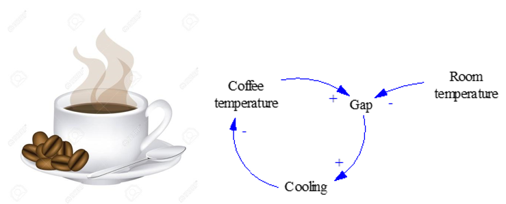
Figure 3: The example of a hot cup of coffee.
What will happen next?
The hot cup of coffee will gradually cool down to equal the room temperature.
The rate of cooling for the cup of coffee (i.e., the speed at which the cup of coffee will cool down) depends on the difference (the “discrepancy”) between the temperature of the coffee and the temperature of the room where you are sitting. In detail, the following stock and flow diagram (Figure 4) depicts this situation (actually, the structure of this system).
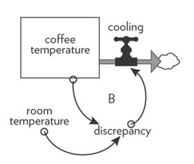
Figure 4: The stock and flow diagram for the system under analysis (“hot cup of coffee”).
Source; Meadows (2008, p. 29).
The greater is the difference between the temperature of the cup of coffee and the temperature of the room (that is to say, the greater is the discrepancy), the faster the coffee will cool.
As an example, imagine starting with a cup of coffee that might have different temperatures, one close to 100°C (i.e., almost boiling) and two others lower than that. The upper part of the following figure (Figure 5) shows what will happen (i.e., the dynamic behavior for this system) starting from different initial values for the coffee and a room temperature which is the same in all the scenarios.
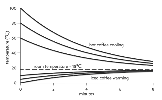
Figure 5: The functioning of the balancing loop in the “hot cup of coffee” system.
Source; Meadows (2008, p. 29).
A balancing loop works to bring the system in equilibrium, that is to say to equal the value of the stock (here, the coffee) and the desired value (i.e., the goal – here the temperature of the room).
Given this discrepancy, the stock will change through its rate to reach the intended goal. Notably, the change is faster at the beginning – when the discrepancy is very high – and slower afterward, as the discrepancy between the two temperatures.
Of course, this will happen if you don’t drink the coffee and just wait!
Notably, the same logic works the other way too, i.e., when you will prepare an iced coffee and the room temperature is high (see Figure 6). The coffee will gradually warm up at a pace that depends on the discrepancy between the temperature of the coffee and the one of the environment.
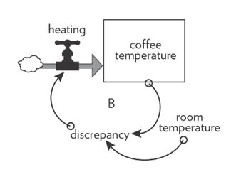
Figure 6: The stock and flow diagram for the “iced cup of coffee” system.
Source; Meadows (2008, p. 29).
The balancing loop, again, works to bring the system in equilibrium with the desired goal, here with the coffee progressively warming up (see the bottom part of Figure 5 for the dynamic behavior).
Positive Feedback Loop coupled with a Negative Feedback loop: limits to growth and epidemic dynamics
Interesting and frequent is the case in which a reinforcing feedback is associated with a balancing one. One can say a reinforcing feedback, which creates an exponential growth (or exponential decay), sooner or later is going to be “limited” by a balancing process. This is coherent with the physical perspective that states that in a limited world nothing can grow forever.
Among other things, it describes every living population and every economy, and the associated structure is called “limits to growth”. In fact, any population has a reinforcing loop causing it to grow through its birth rate, and a balancing loop causing it to die off through its death rate.

Figure 7: The stock and flow diagram for the “population” system.
Source; Meadows (2008, p. 42).
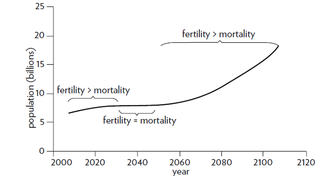
Figure 8: The dynamic behavior over time of the “population” system.
Source; Meadows (2008, p. 47).
The flu contagion process is today another clear example of an exponential self-sustaining process associated with a self-balancing mechanism. In a limited, relatively stable population, the growth in the number of infected people will reach an equilibrium when there are no other individuals who may be infected. Subsequently, as the sick people recover (recovered people) their number decreases to zero. This is called the "SIR model" to indicate the stock variables included, one of the most basic models for describing the temporal dynamics of an infectious disease in a population.
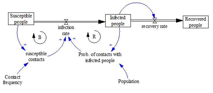
Figure 9: The stock and flow diagram for the “epidemics” system
(elaborated from https://en.wikipedia.org/wiki/Compartmental_models_in_epidemiology).
This is constituted by three main stocks, one related to the population susceptible of being infected, another stock by the infected population, that will increase over time due to the infection process, which is in turn characterized by a rate through which people get infected and thus move from the status of “Susceptible” (one may say also potentially infectable) to the status of having been “Infected” and a third one determining those who have “recovered” from the flu (through a recovery rate)
The fact that people may ignore having been infected (as there typically is a delay between getting infected, developing the illness and the insurgence of the symptoms), would allow them to go around and meet (and potentially infect) those who have not yet been infected (the infection rate thus is based on the contacts between infected and uninfected people).
In the early stages of the epidemics, the number of infected people is low and the number of susceptible is very high: this initially triggers an exponential self-sustaining process in the number of infected people but, in the context of a limited and relatively stable population, such a growth will slow down when there are less opportunities for infecting other individuals (that is, more than 50% of the relevant population has been infected) and will ultimately reach an equilibrium (when potentially everyone of the starting population pool has been infected).
Many know about the famous words used in the news when we are warned about the upcoming “flu-peak”… this is indeed happening when the reinforcing loop (infection rate) reaches its maximum (tipping point) when around 50% of the population has been infected, after which the curve related to infected people starts to slow down.
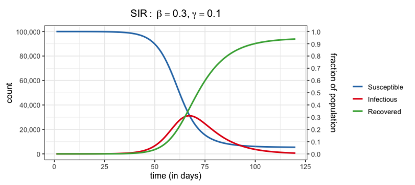
Figure 10: Time graph for the “epidemics” system.
Source; http://people.wku.edu/lily.popova.zhuhadar.
There is a plenty of materials on this topic: for a simple but more exhaustive explanation, for example we do also invite everyone to check: http://people.wku.edu/lily.popova.zhuhadar/
Contributions from: Federico Barnabè, Rocco Scolozzi, Stefano Armenia [SYDIC].
References and further readings
Cavana, R.Y., Mares, E.D. 2004. Integrating critical thinking and systems thinking: from premises to causal loops. System Dynamics Review 20, 223–235. https://doi.org/10.1002/sdr.294
Maani, K. E., & Cavana, R. Y. 2000. Systems thinking and modelling. Understanding change and complexity. Auckland, New Zealand: Prentice Hall.
Meadows D.H. 2008), Thinking in Systems: A primer. Chelsea Green Publishing.
Morecroft, J. D. W., & Sterman, J. D. (Eds.) 2000. Modeling for Learning Organizations, 1st Paperback ed., Portland, OR: Productivity Press.
SIR Model Simply Explained, http://people.wku.edu/lily.popova.zhuhadar/
Wolstenholme, E.F. 2004. Using generic system archetypes to support thinking and modelling. System Dynamics Review 20, 341–356.
Senge, P.M., 1990. The fifth discipline: the art and practice of the learning organization. Doubleday Currency, London.
Sterman, J.D. 2000. Business dynamics. System thinking and modeling for a complex world. Boston: McGraw-Hill.
Senge P.M., Kleiner A., Roberts C., Ross R.B., Smith B.J. 2014. The Fifth Discipline Fieldbook, Strategies and tools for building a learning organization. Currency.

